Atom typing recovery experiment.

Open in Google Colab: http://data.wangyq.net/esp_notebooks/typing.ipynb

(GPU preferred)

In this notebook, we reproduce the atom typing recovery experiment in Wang Y, Fass J, and Chodera JD “End-to-End Differentiable Construction of Molecular Mechanics Force Fields

(Section 3: Graph neural networks can learn to reproduce human-defined legacy atom types with high accuracy; Figure 3. Graph neural networks can reproduce legacy atom types with high accuracy.)

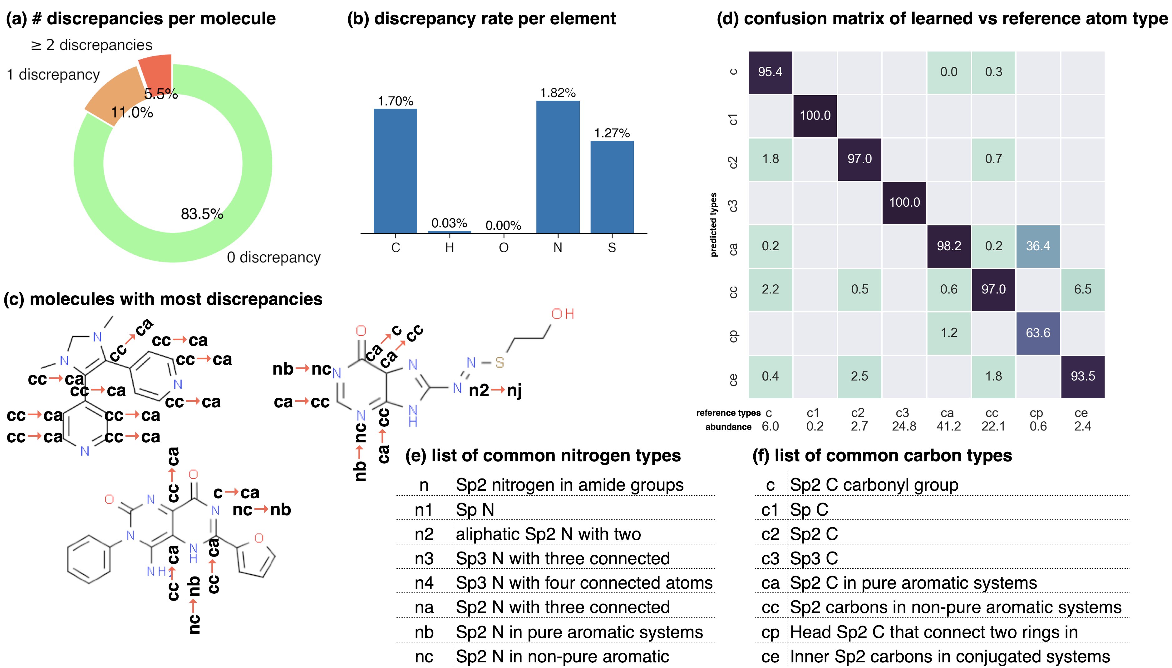
Graph neural networks can reproduce legacy atom types with high accuracy.

The Stage 1 graph neural network of Espaloma chained to a discrete atom type readout was fit to GAFF 1.81 atom types on a subset of ZINC distributed with parm Frosst as a validation set .

The 7529 molecules in this set were partitioned 80:10:10 into training:test:validation sets for this experiment. The overall test set accuracy was $99.07{\mathrm{\%}}_{98.93\mathrm{\%}}^{99.22\mathrm{\%}}$, with 1000 bootstrap replicates used to estimate the confidence intervals arising from finite test set size effects. (a) The distribution of the number of atom type discrepancies on the test set demonstrates that only a minority of atoms are incorrectly typed. (b) The error rate per element is primarily concentrated within carbon, nitrogen, and sulfur types. (c) Examining atom type failures in detail on molecules with the largest numbers of discrepancies shows that the atom types are easily confused by a human, since they represent qualities that are difficult to precisely define. (d) The distribution of predicted atom types for each reference atom type for carbon types are shown; on-diagonal values indicate agreement. The percentages annotated under x-axis denote the relative abundance within the test set.

Installation and Imports

First, we install espaloma after all of its dependencies. Note that this is going to be significantly simplified.

%%capture
! wget -c https://repo.anaconda.com/miniconda/Miniconda3-latest-Linux-x86_64.sh
! bash Miniconda3-latest-Linux-x86_64.sh -b -f -p /usr/local
! conda config --add channels conda-forge --add channels omnia --add channels omnia/label/cuda100 --add channels dglteam
! conda update --yes --all
! conda create --yes -n openmm python=3.6 numpy openmm openmmtools rdkit openforcefield==0.7.0 dgl-cuda10.0 qcportal
! git clone https://github.com/choderalab/espaloma.git

import torch
import dgl
import numpy as np

Get dataset

import os
if not os.path.exists("zinc"):
    os.system("wget data.wangyq.net/esp_datasets/zinc")
ds = esp.data.dataset.GraphDataset.load("zinc")

Assign legacy typing

Next, we assign legacy typings using GAFF-1.81 force field.

typing = esp.graphs.legacy_force_field.LegacyForceField('gaff-1.81')
ds.apply(typing, in_place=True) # this modify the original data

Data massaging

We then split the data into training, test, and validatoin (80:10:10) and batch the the datasets.

ds_tr, ds_te, ds_vl = ds.split([8, 1, 1])

ds_tr = ds_tr.view('graph', batch_size=100, shuffle=True)
ds_te = ds_te.view('graph', batch_size=100)
ds_vl = ds_vl.view('graph', batch_size=100)

Defining model

We define a graph neural network (GNN) model with SAGEConv with 128 units, three layers, and ReLU activation functions.

# define a layer
layer = esp.nn.layers.dgl_legacy.gn("SAGEConv")

# define a representation
representation = esp.nn.Sequential(
        layer,
        [128, "relu", 128, "relu", 128, "relu"],
)

# define a readout
readout = esp.nn.readout.node_typing.NodeTyping(
        in_features=128,
        n_classes=100
)

net = torch.nn.Sequential(
    representation,
    readout
)

Define graph-level loss function

loss_fn = esp.metrics.TypingAccuracy()

Train the model

# define optimizer
optimizer = torch.optim.Adam(net.parameters(), 1e-5)

# train the model
for _ in range(3000):
    for g in ds_tr:
        optimizer.zero_grad()
        net(g.heterograph)
        loss = loss_fn(g.heterograph)
        loss.backward()
        optimizer.step()